
End-to-End Differentiable Models and Optimization for Solid Rocket Powered Aircraft with Plume Radiant Emission
See my published journal paper on this project on AIAA (or find an open access pdf here).
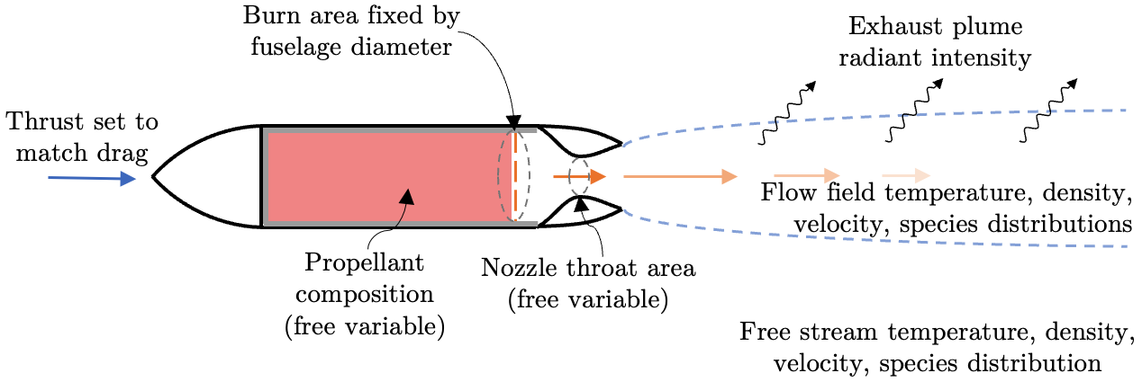
For applications where vehicle visibility is a concern, exhaust plume radiant emission is an important aspect of solid rocket powered vehicle performance. Typical modeling approaches are computationally expensive, and rely on CFD and complicated integration schemes that are not well-suited for fast, iterative vehicle design. To address this gap, I developed simpler models for exhaust plume radiant emission, and implemented them in the fast, flexible AeroSandbox design optimization framework.
During my graduate research at MIT, I worked on a broader research effort to design, build, and characterize propulsion systems for a class of small ( < 10 kg), fast (> 100 m s-1) aircraft. A proposed design for this class of aircraft utilizes a small, end-burning solid rocket motor and a class of slow-burning propellants doped with the burn rate suppressant oxamide, similar to the motors developed, tested, and measured in the static fires described in the exhaust plume radiant emission experiments I conducted. This aircraft concept, illustrated below, will be used as a case study to explore the capabilities of the developed plume radiant emission model.
Design Optimization with CasADi and AeroSandbox
The modeling and optimization work leverages the AeroSandbox framework, a flexible framework for implementing and solving high-dimensional engineering problems including fully- or under-constrained systems of nonlinear, implicit, and differential equations. AeroSandbox solves design problems using the CasADi framework for automatic differentiation. Automatic differentiation is a method for evaluating computational function derivatives by decomposing functions into elementary functions which have known derivatives, and then combining those derivatives using the chain rule. It can be used to compute derivatives for gradient-based optimization schemes and provides a computationally efficient method to solve high-dimensional engineering problems.
I developed and implemented an end-to-end differentiable model for exhaust plume radiant emission (discussed further below) in the AeroSandbox framework. A comparison of the model results to experimental data is shown in the following section.
Model Comparison with Experimental Data
Example 1: Comparison with Small, End-burning Motor Experiments
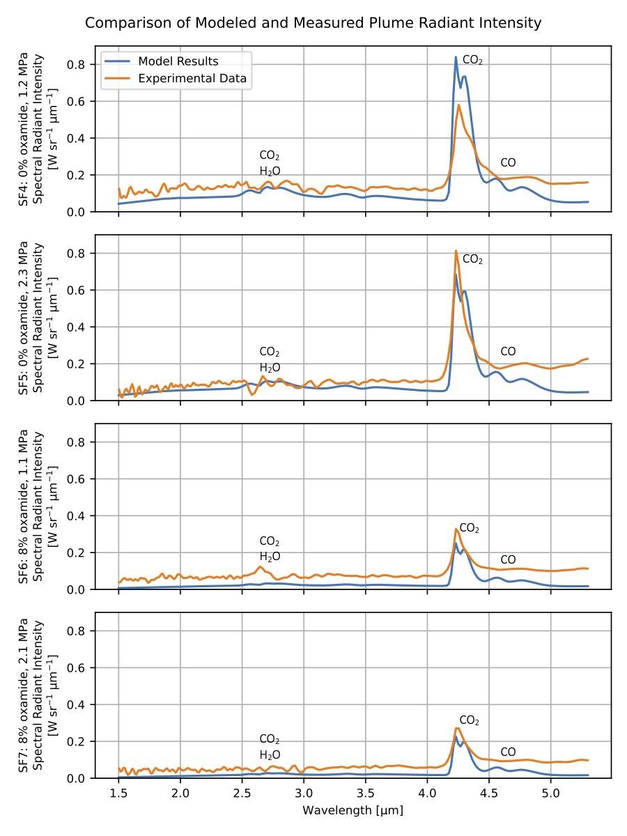
In the figure below is a comparison of model results with the exhaust plume radiant emission measurements collected during the experiments for my graduate research. For all four static fires, both the measured and modeled spectra show a distinct peak at 4.3 μm corresponding to CO2 emission. Weaker emission peaks corresponding to a CO band at 4.7 μm and a combined CO2 and H2O band at 2.7 μm are also present. The measured data and modeled results show reasonable agreement across the spectrum for all four static fires, although the measured experimental data is unfortunately noisy across the spectrum, especially away from the 4.3 μm CO2 peak where the measured signal is weak. Unfortunately, the radiant emission of these small, slow-burning solid rocket motors required operating the radiometric instrumentation near its lower sensitivity limit.
It can be seen in the previous figure that radiant intensity measurements show greater sensitivity to changes in oxamide content than changes in chamber pressure. The modeled radiant intensities display this same trend as well. The reasons for this become more clear by examining the modeled flow field parameters for SF4 - SF7, which are shown in the figure below. Parameters are plotted against axial distance downstream from the start of the turbulent mixing region, normalized by the diameter of the plume \(d_0\) at the start of the turbulent mixing region.
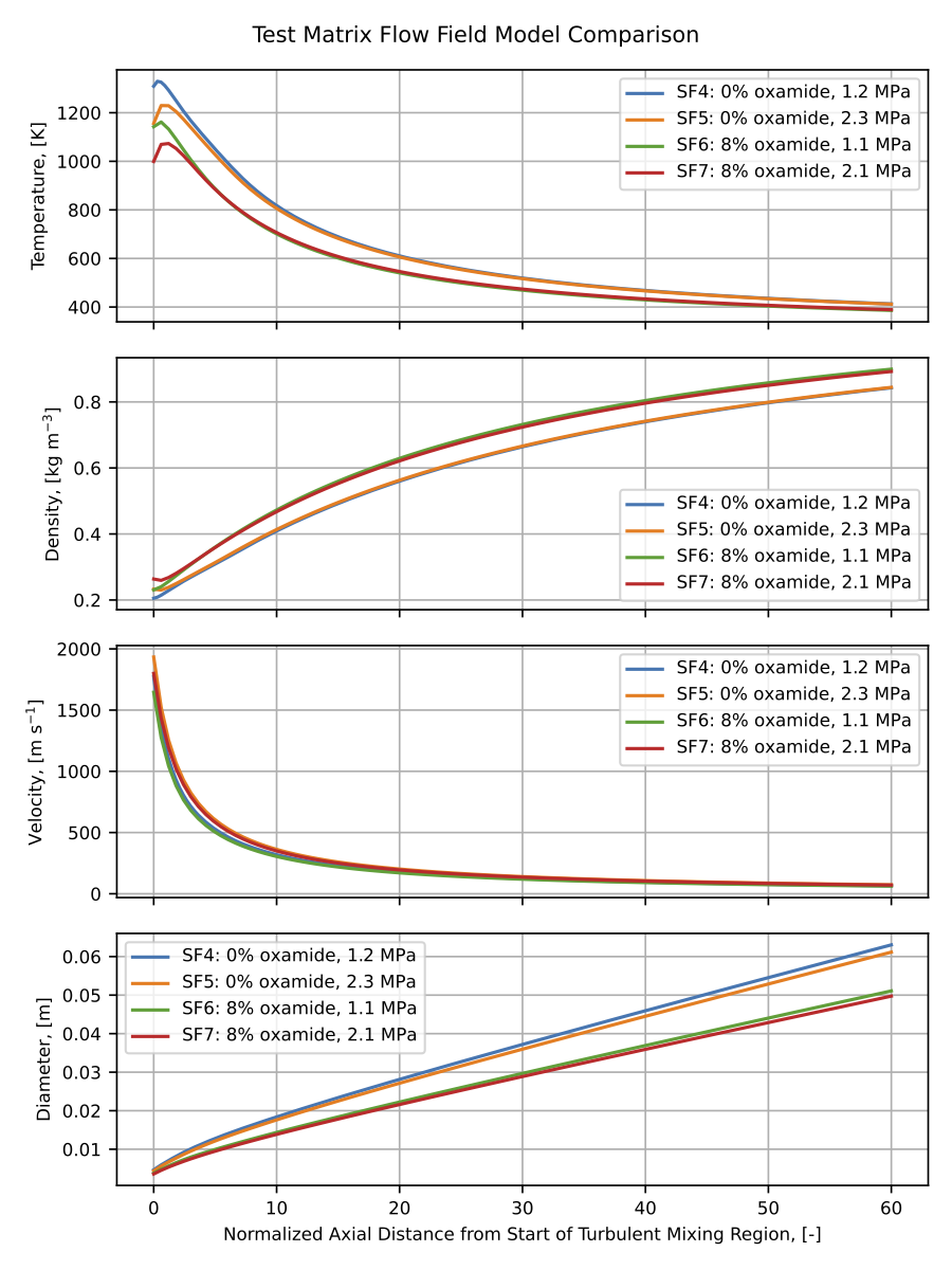
For a given oxamide content (for instance, SF4 and SF5 at 0% oxamide), although a change in chamber pressure causes the flow field properties to separate for a few \(d_0\), they quickly converge to similar values as the plume mixes with entrained air and cools. However, across oxamide contents (SF4 and SF5 at 0% oxamide versus SF6 and SF7 at 8% oxamide) the flow field properties are significantly different throughout the whole flow field, which ultimately leads to significantly different peak radiant intensity values for different oxamide contents.
Example 2: Comparison with Avital et al. Experiment
The developed radiant intensity model was compared to experimental data collected for a small test motor by Avital et al1. The test used a core-burning propellant grain consisting of 87% ammonium perchlorate oxidizer and 13% hydroxyl-terminated polybutadiene binder. The nozzle had a throat diameter of 15 mm, a chamber pressure of 3.8 MPa, and a nozzle exit pressure of 0.27 MPa. The experimental radiant intensity data given by Avital et al. is plotted with the output of the differentiable model in the figure below.
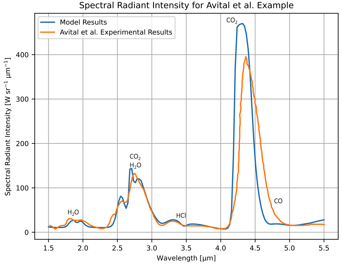
The agreement between the model and the Avital et al. experimental radiant intensity spectra is good. The model performs especially well for the 1.87 μm H2O band, the 2.7 μm combined CO2 and H2O band, and the 3.5 μm HCl band. Some of these bands were not visible in the radiant intensity data or model results for the SF4 - SF7 static fires shown in the previous section due to the low temperatures and small size scales of those plumes. The model over-predicts the 4.3 μm CO2 peak radiant intensity by 19%. The center of the 4.3 μm CO2 band between the model and Avital et al. measurement also differs, with the model predicting the band center near 4.31 μm and the data showing the center near 4.37 μm.
The Avital et al. plume had a peak radiant emission that was over three orders of magnitude larger than the emission from the small end-burning motors discussed in the previous section. The developed radiant emission model performs reasonably well for the Avital et al. plume and the small end-burning plumes, which demonstrates the model’s robustness for modeling plumes spanning multiple orders of magnitude of radiant emission.
General Model Description
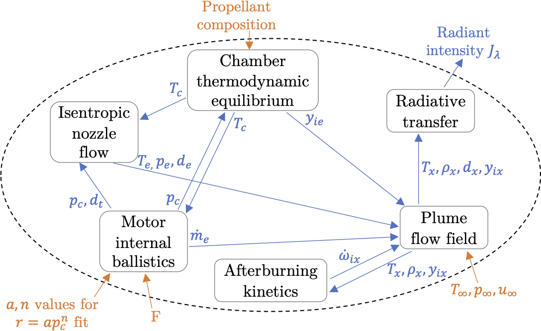
Six end-to-end differentiable sub-models of different coupled physical phenomena were developed and implemented to predict exhaust plume radiant intensity. Their dependencies and information flow are shown in the figure above. These models are summarized here:
-
The chamber thermodynamic equilibrium sub-model predicts the motor combustion chamber temperature \(T_c\) and species mass fractions \(y_{ic}\) given the propellant composition and chamber pressure \(p_c\). This sub-model uses equilibrium thermodynamics calculations.
-
The motor internal ballistics sub-model determines motor equilibrium mass flow, chamber pressure \(p_c\), and nozzle throat diameter \(d_t\) given chamber temperature \(T_c\), propellant \(a\) and \(n\) values, and desired thrust \(F\). These values are solved using a mass flow balance between the burning propellant and the nozzle exit.
-
The isentropic nozzle flow sub-model determines nozzle exit temperature \(T_e\), pressure \(p_e\), and diameter \(d_e\) given chamber temperature \(T_c\), chamber pressure \(p_c\), and nozzle throat diameter \(d_t\). For simplicity, these values are calculated using isentropic nozzle theory assuming frozen flow in the nozzle.
-
The plume flow field sub-model determines temperatures, densities, pressures, and species concentrations throughout the exhaust plume given nozzle exit properties and freestream conditions. A 1D simplified plume flow field model is implemented that captures the core effects of turbulent entrainment, jet expansion, and non-equilibrium chemistry. This 1D model is efficient and compatible with AeroSandbox, and does not rely on black-box CFD codes used by many studies.
-
The afterburning kinetics sub-model determines the species production rates \(\dot{\omega}_i\) throughout the plume given temperatures, densities, and species mass fractions throughout the plume. This sub-model uses a simple, single reaction mechanism with a global reaction rate equation fit to reaction rates predicted by a 28 reaction mechanism. This fitted global reaction rate equation is significantly less stiff than more complicated reaction mechanisms used in other studies, which improves its performance in AeroSandbox.
-
The radiative transfer sub-model determines the plume radiant intensity \(J_{\lambda}\) given temperatures, densities, and species mass fractions throughout the plume. This sub-model integrates the radiative transfer equation along lines-of-sight through the plume, and uses the Ludwig et al. single line group model2 for predicting molecular emission.
Implementation of Design Problems AeroSandbox
Defining Design Problems
All design problems implemented in AeroSandbox are defined as an optimization problem, even if the problem is fully constrained. Standard optimization problems are written using four elements:
-
Variables are quantities in the design problem that are not known; they are degrees of freedom and their values are solved for by the optimizer.
-
Constraints put bounds on variables or expressions that are functions of variables. They constrain the feasible design space. Constraints can be defined as equalities or inequalities.
-
The objective is the function in the design problem that is to be minimized by the optimizer. This is often a relevant performance metric.
-
Parameters are quantities in the design problem that have a pre-selected value that may be changed to update assumptions or perform design sweeps, but are otherwise treated as a constant by the optimizer during any particular optimization.
AeroSandbox provides straightforward syntax for implementing each of these optimization problem elements for a design problem. Each of the sub-models are implemented in separate python classes as fully constrained systems of equations; that is, there are the same number of variables as there are constraints. Fully constrained systems do not need an objective function since the feasible space for solutions is already a single point. The developed models can be assembled into a larger optimization problem with additional variables, constraints, parameters, and an objective if desired.
Model Limitations
Despite its great flexibility, the AeroSandbox framework does create some limitations on the types of models that can be used. The most important of these limitations are described below:
-
Glass-box models: AeroSandbox uses automatic differentiation, which evaluates computational function derivatives by decomposing functions into elementary functions which have known derivatives, and then combining those derivatives using the chain rule. In order to evaluate these derivatives, AeroSandbox needs direct access to the code for the model. Therefore models in AeroSandbox must be “glass-box”, and coded directly in python; “black-box” codes cannot be used.
-
C1-continuity: AeroSandbox uses gradient descent with automatic differentiation to solve optimization problems, which requires that models be C1-continuous with respect to any problem variables. AeroSandbox has several tools for implementing surrogate models to meet the C1-continuity requirement.
-
Non-stiff differential equations: AeroSandbox uses a simple trapezoidal integrator for integrating differential equations. This integrator does not converge well for stiff systems of differential equations, and therefore stiff equations should be avoided.
In Depth Sub-model Implementation Discussion: Chamber Thermodynamic Equilibrium Example
This section will give an in-depth discussion of the chamber thermodynamic equilibrium sub-model as an example. The full code for this sub-model is available on GitHub. A full discussion of all of the sub-models is published with AIAA (or find an open access pdf here).
Propellant combustion temperature and product species fractions are calculated in the chamber thermodynamic equilibrium model. These propellant combustion properties are determined in this model using equilibrium thermodynamics. Namely, combustion temperature and products species mole fractions are determined by minimizing their Gibbs free energy subject to conservation of mass and enthalpy. Which species to include in the combustion products are simply guessed at using the common combustion products for solid rocket propellants (and species that are not present will simply solve to near-zero mole fractions). The implemented governing equations and AeroSandbox implementation methodology are described below.
Governing Equations
The governing equations for the chamber thermodynamic equilibrium module for gaseous products are given below, following the formulation given by Ponomarenko3:
Minimization of Gibbs free energy for gaseous products:
\[\hat{g^0_j}(T_c) + \hat{R} T_c \ln \left(\frac{n_j}{n_{tot}} \right) + \hat{R} T_c \ln \left( \frac{p_c}{p_0} \right) - \sum_{i=1}^{N_{elements}} \lambda_{i} a_{ij} = 0\] \[\text{for } j = 1, \ldots, N_{prod}\]Conservation of mass of chemical elements:
\[\sum_{j=1}^{N_{prod}} a_{ij} n_j - \sum_{k=1}^{N_{reac}} b_{ik} n_k = 0 \hspace{0.3in} \text{for } i = 1, \ldots, N_{elements}\]Conservation of enthalpy:
\[\sum_{j=1}^{N_{prod}} n_j \hat{h}_j^0 - H_0 = 0\]Enforcement of molar sum of gaseous products:
\[\sum_{j=1}^{N_{prod}} n_j - n_{tot} = 0\]The parameters in the governing equations are given in the table below:
| Variable | Python Variable | Description |
|---|---|---|
| \(i\) | i |
chemical elements |
| \(j\) | j |
product species |
| \(k\) | k |
reactant components |
| \(N_{elements}\) | n_elements |
number of chemical elements \(i\) |
| \(N_{prod}\) | n_prod |
number of product species \(j\) |
| \(N_{reac}\) | n_reac |
number of reactant components \(k\) |
| \(T_c\) | temp_c |
chamber temperature [K] |
| \(p_c\) | p_c |
chamber pressure [Pa] |
| \(p_0\) | p_0 |
standard pressure [Pa] |
| \(\hat{g^0_j}\) | g_j |
molar Gibbs free energy of species \(j\) [J mol-1] |
| \(\hat{h^0_j}\) | h_j |
molar enthalpy of species \(j\) [J mol-1] |
| \(\hat{s^0_j}\) | s_j |
molar entropy of species \(j\) [J mol-1 K-1] |
| \(H_0\) | H_0 |
total system enthalpy [J] |
| \(\lambda_{i}\) | lagrange_i |
Lagrange multiplier for element \(i\) |
| \(a_{ij}\) | prod_stoich_coef_mat |
number of atoms of element \(i\) per mole of product species \(j\) |
| \(b_{ik}\) | reac_stoich_coef_mat |
number of atoms of element \(i\) per mole of reactant component \(k\) |
| \(n_j\) | n_j |
number of moles of product species \(j\) |
| \(n_k\) | n_k |
number of moles of reactant component \(k\) |
| \(n_{tot}\) | n_tot |
total number of moles of product species |
| \(\hat{R}\) | R_univ |
universal gas constant [J mol-1 K-1] |
Gibbs free energy can be calculated using \(\hat{g^0_j} = \hat{h^0_j} - T_c \hat{s^0_j}\). Lagrange multipliers \(\lambda_i\) are introduced, following the procedure used by Ponomarenko. Using Lagrange multipliers allows the thermodynamic equilibrium problem to be solved as a system of constrained equations, rather than as a true minimization problem. This is important for implementation in AeroSandbox, so that the equations can be implemented as a set of problem constraints, rather than as a minimization which would be implemented as part of the problem objective.
Implementation in AeroSandbox
The above equations are implemented in python with AeroSandbox. First, we instantiate an AeroSandbox optimization environment:
import aerosandbox as asb
import aerosandbox.numpy as np
opti = asb.Opti()
Next, we identify the problem variables: the number of moles of each product species \(n_j\) (\(N_{prod}\) variables); the total number of moles of gas \(n_{tot}\) (1 variable); the equilibrium combustion temperature \(T_c\) (1 variable); and the Lagrange multipliers \(\lambda_i\) (\(N_{elements}\) variables). These variables are implemented as problem variables. The number of moles of each species \(n_j\) and the lagrange multipliers \(\lambda_i\) are implemented as vectors of variables.
# total number of moles n_tot, assuming 1kg of gas total
# -------------------------
# guess: (1kg) / (a reasonable molecular weight)
n_tot_guess = 1 / .025
n_tot = opti.variable(init_guess=n_tot_guess)

# number of moles of each species n_j
# -------------------------
# guess: equal number of moles
n_j_guess = 1 / n_prod * np.ones(n_prod) * n_tot_guess
n_j = opti.variable(init_guess=n_j_guess)

# lagrange multipliers
# -------------------------
# guess: zeros, it could be anything
lagrange_guess = np.zeros(n_elements)
lagrange_i = opti.variable(init_guess=lagrange_guess)

# chamber temperature
# -------------------------
# guess: 2500 K flame temperature
temp_c = opti.variable(init_guess=2500)
The problem has \(N_{elements} + N_{prod} + 2\) variables. The same number of constraints are required, which are just the governing equations given in the previous section. Differentiable expressions for the species molar enthalpy \(\hat{h^0_j}(T_c)\) and the species molar entropy \(\hat{s^0_j}(T_c)\) with respect to chamber temperature \(T_c\) were implemented using the NASA 9-coefficient polynomial parametrizations4. With the \(\hat{s^0_j}(T_c)\) and \(\hat{h^0_j}(T_c)\) parametrization, Gibbs free energy was defined:
# define Gibbs free energy
# -------------------------
# h_j and s_j are vectors of molar enthalpies and entropies
# corresponding to the species in n_j at temp_c
g_j = h_j - temp_c * s_j
Two matrices were defined to help with the calculations.
First, a matrix prod_stoich_coef_mat, of size \(j \times i\), with each entry \((j, i)\) corresponding to \(a_{ij}\), the number of atoms of element \(i\) per mole of product species \(j\).
Second, a matrix reac_stoich_coef_mat, of size \(k \times i\), with each entry \((k, i)\) corresponding to \(b_{ik}\), the number of atoms of element \(i\) per mole of reactant component \(k\).
The governing equations were vectorized and enforced as constraints on the opti instance:
# minimize Gibbs free energy for product species
# -------------------------
# combine summation operation into matrix multiplication
# operation ('@' implements matrix multiplication)
opti.subject_to(
    g_j  +
    R_univ * temp_c * np.log(n_j / n_tot) +
    R_univ * temp_c * np.log(p_c / p_0) -
    (prod_stoich_coef_mat @ lagrange_i)
    == 0
)

# conservation of mass for each element
# -------------------------
# assuming arbitrarily 1 kg system mass
# assuming reactant mole fractions n_k are known
opti.subject_to(
    (prod_stoich_coef_mat.T @ n_j) -
    (reac_stoich_coef_mat.T @ n_k)
    == 0
)

# conservation of total enthalpy in reacting system
# -------------------------
# assumes H_0 is known and calculated from known
# reactant mole quantities n_k
opti.subject_to(np.sum(n_j * h_j) - H_0 == 0)

# sum of all n_j equals n_tot
# -------------------------
opti.subject_to(np.sum(n_j) - n_tot == 0)
There are as many enforced constraints as variables: the minimization of Gibbs free energy provides one constraint per product species (\(N_{prod}\) constraints); the conservation of mass for each element provides one constraint per element (\(N_{elements}\) constraints); the conservation of total enthalpy in the reacting system provides one constraint; and the summation of moles provides one constraint. Because there are equal numbers of variables and constraints, an objective is not required for this sub-model, since the solution space is already only a single point. This chamber thermodynamic equilibrium sub-model can be attached to other sub-models, and other constraints can be applied to the entire optimization problem.
Integrated Design of Small, Low-Thrust Solid Rocket Motors Including Plume Radiant Emission
Consider an example of integrated design of a solid rocket powered aircraft using the complete model for radiant emission (all six sub-models). For the example, we choose the proposed design for a small, fast aircraft described at the top of this post. The aircraft utilizes a small, end-burning solid rocket motor and a class of slow-burning propellants doped with the burn rate suppressant oxamide. This aircraft concept is illustrated in the figure below (same figure as at the top of this post).
The propellant burn area is fixed by the fuselage diameter. The propellant composition is a free variable, but is constrained as a baseline propellant that can be diluted with some mass fraction of oxamide. The throat diameter is a free variable, and its value ultimately sets the chamber pressure. The thrust is set to match vehicle drag or some other requirement.
The following parameters are chosen:
- 2500 mm2 propellant burning area
- 10 km altitude
- Mach 0.8 vehicle speed
- matched nozzle expansion
- viewing orthogonal to plume axis of symmetry
Thrust and oxamide content are set as problem parameters in AeroSandbox, and are swept through reasonable values. The system is solved for chamber pressure and nozzle throat diameter. The resulting radiant intensity, chamber pressure, and specific impulse for each of these configurations are plotted in the design chart below for curves of constant thrust.
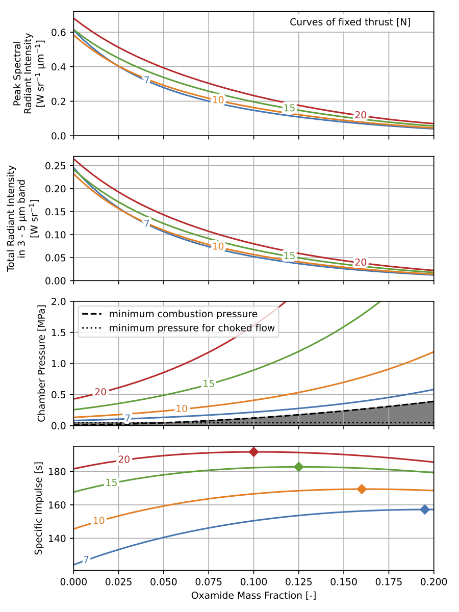
This design chart helps to characterize the trade-offs between aircraft thrust, propellant oxamide content, chamber pressure, and plume radiant intensity. For a particular aircraft thrust, a range of radiant intensities can be achieved by operating at different oxamide contents and chamber pressures. Operating at higher propellant oxamide content yields lower radiant intensities. For a particular propellant oxamide mass fraction, the radiant intensity cannot be changed significantly by changing the chamber pressure. A different combination of oxamide content and chamber pressure maximizes the specific impulse for each aircraft thrust.
Much of the discussion on this page was borrowed from my PhD thesis.
-
G. Avital et al. “Experimental and Computational Study of Infrared Emission from Underexpanded Rocket Exhaust Plumes”. In: Journal of Thermophysics and Heat Transfer 15.4 (Oct. 2001), pp. 377 - 383. issn: 0887-8722, 1533-6808. ↩
-
C. B. Ludwig et al. Handbook of Infrared Radiation from Combustion Gases. NASA SP-3080. NASA Marshall Space Flight Center, 1973. ↩
-
Alexander Ponomarenko. “RPA: Tool for Liquid Propellant Rocket Engine Analysis C++ Implementation”. In: (2010), p. 23. ↩
-
Bonnie J. McBride, Michael J. Zehe, and Sanford Gordon. NASA Glenn Coefficients for Calculating Thermodynamic Properties of Individual Species. NTRS Author Affiliations: NASA Glenn Research Center NTRS Report/Patent Number: NASA/TP-2002-211556 NTRS Document ID: 20020085330 NTRS Research Center: Glenn Research Center (GRC). Sept. 1, 2002. ↩